Train a PINN (Physics Informed Neural Network) Shrodinger equation

Shrodinger equation is a classical field equation used to study quantum mechanical systems, including nonlinear wave propagation in optical fibers.

It is a complex one-dimensional nonlinear equation. In this example the the nonlinear Schrödinger equation along with periodic boundary conditions is guven by

\[i h_t + 0.5 h_{xx} + |h|^2 h = 0, \quad x \in [-5, 5], \quad t \in [0, \pi/2],\]

\[h(0, x) = 2 \, \text{sech}(x),\]

\[h(t, -5) = h(t, 5), h_x(t, -5) = h_x(t, 5)\]

This example has been extracted from: https://doi.org/10.1016/j.jcp.2018.10.045 .M. Raissi, P. Perdikaris, G.E. Karniadakis

Physics-informed neural networks: A deep learning framework for solving forward and inverse problems involving nonlinear partial differential equations

from cetaceo.models import MLP
from cetaceo.models.pinn import BoundaryCondition
from cetaceo.models.pinn import PINN
from cetaceo.pipeline import Pipeline
from cetaceo.evaluators import RegressionEvaluatorPlotter
from cetaceo.plotting import TrueVsPredPlotter
from cetaceo.data import TorchDataset

import numpy as np
import scipy.io
from scipy.interpolate import griddata
import torch

import matplotlib.gridspec as gridspec
import matplotlib.pyplot as plt
import time
from mpl_toolkits.axes_grid1 import make_axes_locatable
from pathlib import Path

# Latin Hypercube sample defined to generate Collocation points
def lhs(n, samples):
    # Generate the intervals
    cut = np.linspace(0, 1, samples + 1)

    # Fill points uniformly in each interval
    u = np.random.rand(samples, n)
    a = cut[:samples]
    b = cut[1:samples + 1]
    rdpoints = np.zeros_like(u)
    for j in range(n):
        rdpoints[:, j] = u[:, j]*(b-a) + a

    # Make the random pairings
    H = np.zeros_like(rdpoints)
    for j in range(n):
        order = np.random.permutation(range(samples))
        H[:, j] = rdpoints[order, j]

    return H

device = 'cuda' if torch.cuda.is_available() else 'cpu'

DATA_DIR = Path.cwd() / "Data"
CASE_DIR = Path.cwd() / "results"

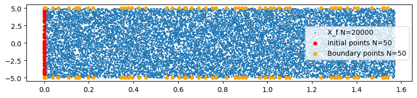
Define BC points and Collocation points

The number of initial points is N_0=50, boundary points N_b=50 and Collocation points N_f=20000.

The real data is going to be impossed in the initial and boundary condition, it is read from the NLS.mat file. This mat file can be found at https://github.com/maziarraissi/PINNs/tree/master/main/Data

#Domain bounds
lb = np.array([-5.0,-0.0])      #bottom left domain point
ub = np.array([5.0, np.pi/2])   #top right domain point

N_0 = 50
N_B = 50
N_F = 20000

#Obtain real data
data = scipy.io.loadmat(DATA_DIR /"NLS.mat")

#Organize data
t = data['tt'].flatten()[:,None]
x = data['x'].flatten()[:,None]
Exact = data['uu']
Exact_u = np.real(Exact)
Exact_v = np.imag(Exact)
Exact_h = np.sqrt(Exact_u**2 + Exact_v**2)

X, T = np.meshgrid(x,t)

X_star = np.hstack((X.flatten()[:,None], T.flatten()[:,None]))
u_star = Exact_u.T.flatten()[:,None]
v_star = Exact_v.T.flatten()[:,None]
h_star = Exact_h.T.flatten()[:,None]

#choose N_0 random points of input
idx_x = np.random.choice(x.shape[0], N_0, replace=False)
x0 = x[idx_x,:]
u0 = Exact_u[idx_x,0:1]
v0 = Exact_v[idx_x,0:1]

#choose N_B random points from input
idx_t = np.random.choice(t.shape[0], N_B, replace=False)
tb = t[idx_t,:]

#create collocation points
X_f = lb + (ub-lb)*lhs(2, N_F)

# plot used points
fig, ax = plt.subplots(figsize=(10, 2))
ax.scatter(X_f[:,1], X_f[:,0],label=f"X_f N={N_F}", s=1)
ax.scatter(np.zeros(len(x0)),x0,marker= 'o',color='red',label=f"Initial points N={N_0}",s=20)
ax.scatter(tb,np.full(len(tb), 5.0),marker='o',color='orange',label = f"Boundary points N={N_B}",s=20)
ax.scatter(tb,np.full(len(tb), -5.0),marker='o',color='orange',s=20)
ax.legend(loc='center right')
plt.savefig(CASE_DIR / f'plots/X_f')

Define PDE loss function

It is important to be consistent with the dimensionality of the arrays. In other words, if the user is using columns, all the arrays created in the loss functions has to be columns too.

class ShrodingerPINN(PINN):
    def __init__(self, *args, **kwargs):
        super().__init__(*args, **kwargs)

    def pde_loss(self, pred, *input_variables):

        x,t = input_variables

        u, v = pred[:,0:1], pred[:,1:2]

        u_x = torch.autograd.grad(u, x, grad_outputs=torch.ones_like(u), create_graph=True)[0]
        v_x = torch.autograd.grad(v, x, grad_outputs=torch.ones_like(v), create_graph=True)[0]

        u_t = torch.autograd.grad(u, t, grad_outputs=torch.ones_like(u), create_graph=True)[0]
        u_xx = torch.autograd.grad(u_x, x, grad_outputs=torch.ones_like(u_x), create_graph=True)[0]

        v_t = torch.autograd.grad(v, t, grad_outputs=torch.ones_like(u), create_graph=True)[0]
        v_xx = torch.autograd.grad(v_x, x, grad_outputs=torch.ones_like(u_x), create_graph=True)[0]

        f_u = u_t + 0.5 * v_xx + (u**2 + v**2)*v
        f_v = v_t - 0.5 * u_xx - (u**2 + v**2)*u

        return (f_u ** 2).mean() + (f_v ** 2).mean()

Define Boundary conditions

class InitialCondition(BoundaryCondition):
    def __init__(self, points, value_at_points):
        super().__init__(points)
        self.u = value_at_points[:,0:1].to(device) #!Be carful that arrays are columns
        self.v = value_at_points[:,1:2].to(device) #!Be carful that arrays are columns

    def loss(self, pred):
        u, v = self.u , self.v

        u_pred = pred[:,0:1]
        v_pred = pred[:,1:2]

        return ((u_pred-u)**2).mean() + ((v_pred - v)**2).mean()


class XBoudaryCondition(BoundaryCondition):
    def __init__(self, points):
        super().__init__(points)

    def loss(self, pred):
        u_pred = pred[:,0:1]
        v_pred = pred[:,1:2]

        #Derivatives, this is important to do before any manipulation of vectors.
        u_pred_x = torch.autograd.grad(u_pred,self.points,grad_outputs=torch.ones_like(u_pred),create_graph=True)[0]
        v_pred_x = torch.autograd.grad(v_pred,self.points,grad_outputs=torch.ones_like(u_pred),create_graph=True)[0]

        #Values at upper boundary
        ub_u_pred = pred[:len(pred)//2,0:1]
        ub_v_pred = pred[:len(pred)//2,1:2]

        #Values at lower boundary
        lb_u_pred = pred[len(pred)//2:,0:1]
        lb_v_pred = pred[len(pred)//2:,1:2]

        ub_u_pred_x = u_pred_x[:len(u_pred_x)//2]
        ub_v_pred_x = v_pred_x[:len(u_pred_x)//2]

        lb_u_pred_x = u_pred_x[len(u_pred_x)//2:]
        lb_v_pred_x = v_pred_x[len(u_pred_x)//2:]


        # as u on the boundary is 0, we can just return the mean of the prediction
        return ((ub_u_pred - lb_u_pred)**2).mean() + ((ub_v_pred - lb_v_pred)**2).mean() + ((ub_u_pred_x - lb_u_pred_x)**2).mean() + ((ub_v_pred_x - lb_v_pred_x)**2).mean()

The inital points are defined from x0 and t is full of 0. While the boundary points are different tb points for x = 5 and x = -5.

#BC Definition

x0_ = torch.tensor(x0.reshape(-1, 1))
u0_ = torch.tensor(u0.reshape(-1, 1))
v0_ = torch.tensor(v0.reshape(-1, 1))


initial_bc = InitialCondition(
    torch.cat([x0_, torch.full_like(x0_, 0)], dim=-1).float(),    # [x0, 0]
    torch.cat([u0_, v0_], dim=-1).float()                         # [u0, v0]
)


tb_ = torch.tensor(tb).reshape(-1, 1)
boundary_bc = XBoudaryCondition(
    torch.cat(
        [torch.cat([ torch.full_like(tb_,  5), tb_ ], dim=-1),  # [5,tb]
         torch.cat([ torch.full_like(tb_, -5), tb_ ], dim=-1),] # [-5,tb]
    ).float()
)

Create Dataset

train_dataset = TorchDataset(X_f)

PINN and NN definiton

input_dim = X_f.shape[1]
output_dim = 2 # u(t, x), v(t,x),

net = MLP(
    input_size=input_dim,
    output_size=output_dim,
    hidden_size=100,
    n_layers=5,
    activation=torch.nn.functional.tanh, # With relu the model struggles to converge
)

shrodinger_pinn = ShrodingerPINN(
    neural_net=net,
    device=device,
)

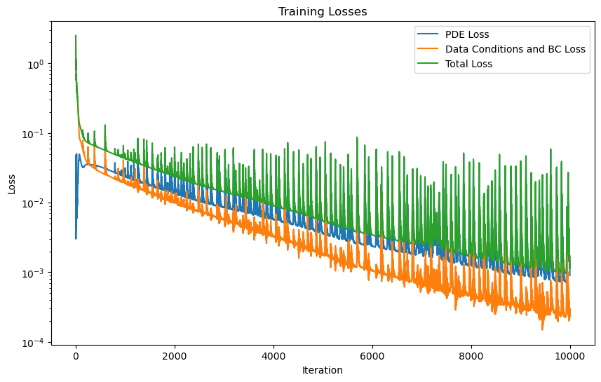
PINN training with Adam optimizer

training_params = {
    'optimizer_class': torch.optim.Adam,
    'optimizer_params': {'lr': 1e-3},
    'epochs': 10000,
    'boundary_conditions': [ initial_bc, boundary_bc],
    'print_every': 1000,
}

pipeline_adam = Pipeline(
    model=shrodinger_pinn,
    train_dataset=train_dataset,
    training_params=training_params,
)

start = time.time()
model_logs = pipeline_adam.run()
end = time.time()
print("training time ADAM: ", end-start)

shrodinger_pinn.plot_training_logs(model_logs)

Epoch 1/10000 Iteration 0. Pde loss: 4.7672e-02, data/bc losses: [1.1603e+00, 1.2829e+00]: 100%|██████████| 1/1 [00:11<00:00, 11.97s/it]
Epoch 1000/10000 Iteration 0. Pde loss: 2.8017e-02, data/bc losses: [1.9799e-02, 1.1357e-03]: 100%|██████████| 1/1 [00:00<00:00, 23.31it/s]
Epoch 2000/10000 Iteration 0. Pde loss: 3.2303e-02, data/bc losses: [1.1159e-02, 9.9579e-04]: 100%|██████████| 1/1 [00:00<00:00, 19.80it/s]
Epoch 3000/10000 Iteration 0. Pde loss: 8.4737e-03, data/bc losses: [5.6386e-03, 7.1361e-05]: 100%|██████████| 1/1 [00:00<00:00, 24.52it/s]
Epoch 4000/10000 Iteration 0. Pde loss: 5.7364e-03, data/bc losses: [3.3060e-03, 6.9943e-05]: 100%|██████████| 1/1 [00:00<00:00, 21.94it/s]
Epoch 5000/10000 Iteration 0. Pde loss: 3.6267e-03, data/bc losses: [1.7787e-03, 5.7431e-05]: 100%|██████████| 1/1 [00:00<00:00, 24.47it/s]
Epoch 6000/10000 Iteration 0. Pde loss: 2.4194e-03, data/bc losses: [1.0164e-03, 3.7985e-05]: 100%|██████████| 1/1 [00:00<00:00, 22.60it/s]
Epoch 7000/10000 Iteration 0. Pde loss: 4.2973e-03, data/bc losses: [5.7286e-04, 3.3943e-05]: 100%|██████████| 1/1 [00:00<00:00, 25.45it/s]
Epoch 8000/10000 Iteration 0. Pde loss: 1.5579e-03, data/bc losses: [5.1239e-04, 5.0528e-05]: 100%|██████████| 1/1 [00:00<00:00, 25.19it/s]
Epoch 9000/10000 Iteration 0. Pde loss: 7.1868e-03, data/bc losses: [1.9607e-04, 1.4594e-04]: 100%|██████████| 1/1 [00:00<00:00, 26.06it/s]
Epoch 10000/10000 Iteration 0. Pde loss: 8.9741e-04, data/bc losses: [2.2386e-04, 1.1224e-05]: 100%|██████████| 1/1 [00:00<00:00, 19.52it/s]

training time ADAM:  422.57659339904785

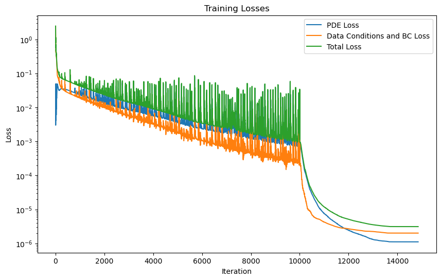
PINN training with LBFGS optimizer

evaluator2 = RegressionEvaluatorPlotter(plots_path=CASE_DIR / 'plots/', plotters=[TrueVsPredPlotter()])
lbfgs_params = {
    'max_iter': 12000,#12000
    'max_eval': 10000,
    'history_size': 200,
    'tolerance_grad': 1e-8,
    'tolerance_change': 1.0 * np.finfo(float).eps,
    # 'line_search_fn': 'strong_wolfe'
}
training_params = {
    'optimizer_class': torch.optim.LBFGS,
    'optimizer_params': lbfgs_params,
    'loaded_logs': model_logs,
    'epochs': 1,
    'boundary_conditions': [initial_bc, boundary_bc], #initial_bc,
}

pipeline_lbfgs = Pipeline(
    model=shrodinger_pinn,
    train_dataset=train_dataset,
    # test_dataset=test_dataset,
    training_params=training_params,
    evaluators=[evaluator2]
)

start = time.time()
model_logs = pipeline_lbfgs.run()
end = time.time()
print("training time ADAM: ", end-start)
shrodinger_pinn.plot_training_logs(model_logs)

Epoch 1/1 Iteration 4800. Pde loss: 1.1083e-06, data/bc losses: [1.9058e-06, 9.8313e-08]: 100%|██████████| 1/1 [04:33<00:00, 273.63s/it]

training time ADAM:  273.63641357421875

pred = shrodinger_pinn.predict(torch.tensor(X_star).float())
u_pred, v_pred = pred[:,0:1], pred[:,1:2]
h_pred = np.sqrt(u_pred**2 + v_pred**2)

H_pred = griddata(X_star, h_pred.flatten(), (X, T), method='cubic')

H_star = griddata(X_star,h_star.flatten(), (X,T), method='cubic')

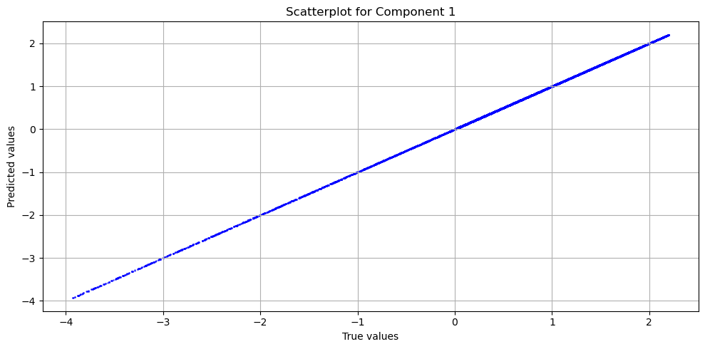
evaluator = RegressionEvaluatorPlotter(plots_path='.', plotters=[TrueVsPredPlotter()])
evaluator(u_pred.reshape(-1, 1), u_star.reshape(-1, 1))
evaluator.print_metrics()

Regression evaluator metrics:
mse: 1.3665e-06
mae: 9.5476e-04
mre: 0.8756%
ae_95: 0.0022
ae_99: 0.0028
r2: 1.0000
l2_error: 0.0017

gs1 = gridspec.GridSpec(1, 3)
gs1.update(top=1-1/3, bottom=0, left=0.1, right=0.9, wspace=0.5)

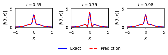
ax = plt.subplot(gs1[0, 0])
ax.plot(x,Exact_h[:,75], 'b-', linewidth = 2, label = 'Exact')
ax.plot(x,H_pred[75,:], 'r--', linewidth = 2, label = 'Prediction')
ax.set_xlabel('$x$')
ax.set_ylabel('$|h(t,x)|$')
ax.set_title(f'$t = {t[75].item():.2f}$', fontsize=10)
ax.axis('square')
ax.set_xlim([-5.1,5.1])
ax.set_ylim([-0.1,5.1])

ax = plt.subplot(gs1[0, 1])
ax.plot(x,Exact_h[:,100], 'b-', linewidth = 2, label = 'Exact')
ax.plot(x,H_pred[100,:], 'r--', linewidth = 2, label = 'Prediction')
ax.set_xlabel('$x$')
ax.set_ylabel('$|h(t,x)|$')
ax.axis('square')
ax.set_xlim([-5.1,5.1])
ax.set_ylim([-0.1,5.1])
# Asegúrate de que t[100] sea un número real, por ejemplo usando float()
ax.set_title(f'$t = {t[100].item():.2f}$', fontsize=10)
ax.legend(loc='upper center', bbox_to_anchor=(0.5, -0.8), ncol=5, frameon=False)

ax = plt.subplot(gs1[0, 2])
ax.plot(x,Exact_h[:,125], 'b-', linewidth = 2, label = 'Exact')
ax.plot(x,H_pred[125,:], 'r--', linewidth = 2, label = 'Prediction')
ax.set_xlabel('$x$')
ax.set_ylabel('$|h(t,x)|$')
ax.axis('square')
ax.set_xlim([-5.1,5.1])
ax.set_ylim([-0.1,5.1])
# Asegúrate de que t[100] sea un número real, por ejemplo usando float()
ax.set_title(f'$t = {t[125].item():.2f}$', fontsize=10)

Text(0.5, 1.0, '$t = 0.98$')

X0 = np.concatenate((x0, 0*x0), 1) # (x0, 0)
X_lb = np.concatenate((0*tb + lb[0], tb), 1) # (lb[0], tb)
X_ub = np.concatenate((0*tb + ub[0], tb), 1) # (ub[0], tb)
X_u_train = np.vstack([X0, X_lb, X_ub])

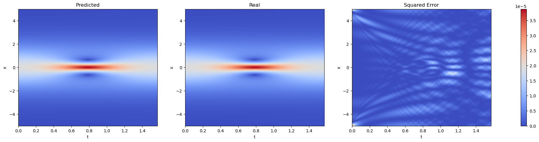
fig, axs = plt.subplots(1, 3, figsize=(25, 5))
for i, (data, title) in enumerate(zip([H_star, H_pred, (H_pred - H_star) ** 2], ['Predicted', 'Real', 'Squared Error'])):
    im = axs[i].imshow(data.T, extent=[lb[1], ub[1], lb[0], ub[0]], origin='lower', aspect='auto', cmap='coolwarm')
    axs[i].set_title(title)
    axs[i].set_xlabel('t')
    axs[i].set_ylabel('x')
    axs[i].set_aspect('auto')
    axs[i].grid(False)

fig.colorbar(im, ax=axs.ravel().tolist())
plt.show()

Save model

print("Saving model")
shrodinger_pinn.save(CASE_DIR / 'models/shrodinger_pinn.pth')
print("Model saved")
shrodinger_pinn_loaded = ShrodingerPINN.load(CASE_DIR / 'models/shrodinger_pinn.pth', device=device)

print("Model loaded")
predictions = shrodinger_pinn_loaded.predict(torch.tensor(X_star).float())
u_pred, v_pred = pred[:,0:1], pred[:,1:2]
h_pred = np.sqrt(u_pred**2 + v_pred**2)

error_u = np.linalg.norm(u_star-u_pred,2)/np.linalg.norm(u_star,2) * 100
error_v = np.linalg.norm(v_star-v_pred,2)/np.linalg.norm(v_star,2) * 100
error_h = np.linalg.norm(h_star-h_pred,2)/np.linalg.norm(h_star,2) * 100

print('Mean Relative Error u: %e ' % (error_u))
print('Mean Relative Error v: %e ' % (error_v))
print('Mean Relative Error h: %e ' % (error_h))

Saving model
Model saved
Model loaded
Mean Relative Error u: 1.657814e-01
Mean Relative Error v: 2.100694e-01
Mean Relative Error h: 1.325840e-01